How to Use Machine Learning to Predict the Quality of Wines

Table of Contents

You can read this same article in Free Code Camp’s Medium Publication.

---

Machine Learning (ML) is a sub-field of artificial intelligence. It concerns giving computers the ability to learn without being explicitly programmed. Over the years, machine learning's popularity and demand has certainly been on the rise, as indicated by this hype curve:

According to Indeed, the average salary for a machine learning engineer in the United States is $134,655. But what is so special about it that it’s one of the highest paid jobs in programming? This article will help you understand its wide array of applications.

This tutorial kicks off from the last one, which shows how you can use Data Science to understand what makes wine taste good! If you haven’t done it already, do check it out first, and you’ll get a fair glimpse of what Data Science is all about -

Using Data Science to Understand What Makes Wine Taste Good

Machine Learning is often the next step in the pipeline, right after Data Science. Ready to be part of the hype? Keep reading!

What is Machine Learning?

In the real world we have humans, and we have computers. How do we humans learn? It’s simple — from past experiences!

Now, we humans use our sensory inputs such as eyes, ears, or sense of touch to get data from our surroundings. We then use this data in a lot of interesting and meaningful ways. Most commonly, we use it to make accurate predictions about the future. In other words, we learn.

For example, is it going to rain this time of the year? Is your girlfriend going to get mad if you forget her birthday? Should you stop when the traffic sign’s red? Should you invest in a piece of real estate? How likely is Jon Snow to survive in the next season of Game of Thrones? To answer these questions, you need past data!

Computers — on the other hand — traditionally don’t use data in the same way that we do. They need to be given a specific set of instructions to follow — in other words, an algorithm. A computer is very good at following a sequence of steps in a short time.

Now the question is — can computers learn from past experiences (or data), just like humans? Yes — you can give them the ability to learn and predict future events, without being explicitly programmed. And that’s precisely what Machine Learning is all about. From self-driving cars, to discovering planets — the applications of ML are immense.

I also read a really nice post on the difference between Data Science, Machine Learning and Artificial Intelligence. It’s a pretty comprehensive one, so I’ll summarize it —

• Data Science produces insights
• Machine Learning produces predictions
• Artificial Intelligence produces actions

And there are lot of overlaps between these fields, which is why these terms are often used interchangably.

When you’re fundraising, it’s AI
When you’re hiring, it’s ML
When you’re implementing, it’s linear regression
When you’re debugging, it’s printf()

— Baron Sc​hwartz (@xaprb) November 15, 2017

At Netflix, Machine Learning is used to learn from data that contains users’ behavioral profiles and shows you good recommendations. Google Search is tailored to show results that are most relevant to you — again with a lot of ML techniques continuously learning from data behind the scenes. In the land of Data Science and ML, data is gold. As Tyrion Lannister might say, if faced with the world of ML and AI:

A company needs data as a sword needs a whetstone, if it is to keep its edge.

Now that we have understood what it’s all about, it’s time to dive in!

Who should read this tutorial:

If you wish to understand machine learning, but have been put off because you find maths, statistics, and implementing algorithms from scratch too complex, then this tutorial is for you.

At some point in your learning, you will need to dive in deeper — you can’t shy away from math for too long! By the end of this article, I hope you’ll be motivated to explore every depth of this field.

If you have some knowledge of programming in Python, and have finished the earlier tutorial, you’re good to go.

Let’s Get Started!

You’ve learned quite a lot about your wines from the previous tutorial. This time, your machine will do the learning. You’ll learn to build a machine learning model, which, if you gave it wine attributes, would accurately tell you how good the wine is. After finishing this tutorial, you’ll get an understanding of:

• Different ML algorithms and techniques
• How to train and build a classifier
• Common errors that occur while building ML models, and how to get rid of them
• How to analyze and interpret the performance of your models

Types of Machine Learning

Supervised Learning

This is what we’ll learn in this tutorial. As the name suggests, Supervised Learning needs a human to “supervise” and tell the computer what it should be trained to predict for, or give it the right answer. We feed the computer with training data containing various features, and we also tell it the right answer.

To give an analogy, imagine the computer to be a kid who’s a blank slate ¹. He knows nothing.

Now, how do you teach Jon Snow the difference between a dog and a cat? It’s quite intuitive — you take him out for a walk, and when you see a cat, you point it out and say, “This is a Cat.” As you keep walking you might see a dog, so you again point it out and say “This is a Dog.” Over time, as you keep showing lots of dogs and cats, the kid will learn to differentiate between the two.

Of course, you can always show Jon lots of pics of dogs and cats instead of going out for a walk. Instagram to the rescue! :P

With respect to our wine data-set, our machine learning model will learn to co-relate between the quality of the wines, versus the rest of the attributes. In other words, it’ll learn to identify patterns between the features and the targets (quality).

Unsupervised Learning

Here we don’t give the computer a “target” label to predict. Instead, we let the computer discover patterns on its own, and then choose the one that makes most sense. This technique is necessary, since often we don’t even know what we are looking for in our data.

Reinforcement Learning

It is used for training an AI agent to “behave” and learn to choose the best action for a given scenario, based on rewards and feedback. It has a lot of parallels with AI.

Apart from these three, there are other types of ML too, like Semi-supervised Learning, clustering etc.

What problems can Supervised Learning solve?

Broadly speaking, supervised ML can be used to solve two types of problems:

Classification

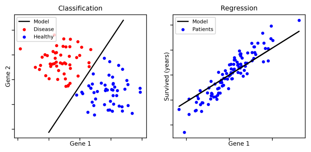
Where you need to categorize a certain observation into a group. In the above picture, if you’re given a dot you need to classify it as either a blue dot or a red dot. Few more examples would be — to predict if a given email is spam or not spam? Is a detected particle a Higgs Boson or a normal sub-atomic particle? Or even assigning a certain news article into a group — like sports, weather, or science.

Regression

Again used for predicting and forecasting, but for continuous values. For example, consider you’re a real estate agent who wants to sell a house that is 2000 sq.feet, has 3 bedrooms, has 5 schools in the area. What price should you sell the house for?

---

A scenario where you need to identify benign tumor cells vs malignant tumor cells would be a classification problem. So the job of the machine learning classifier would be to use the training data to learn, and find this line, curve, or decision boundary that most efficiently separates the two classes.

Note that classification problems need not necessarily be binary — we can have problems with more than 2 classes.

On the other hand, a scenario where you need to determine the life expectancy of cancer patients would be a regression problem. In this case, our model would have to find a line or curve that generalizes really well for most of the data points.

A few regression problems can be transformed into a classification problem as well. Moreover, certain kinds of problems could very well belong to both types, classification as well as regression.

The Mechanism of Machine Learning

Most problems in Supervised Learning can be solved in three stages:

Step #1: Data preparation, transforms and splitting

The first step is to analyze the data and prepare it to be used for training purposes. You observe things like how skewed it is, how well is it distributed, and statistics like mean and median of the features. We already covered this in the earlier blog.

Once you understand them, you can preprocess them and apply feature transformations to it if necessary.

Next, you divide the data into two sets — a bigger chunk for training, and the other smaller chunk for testing. Our classifier will use the training data-set to “learn”. We need a separate chunk of data for testing and validation, so that we can see how well our model works on data that it hasn’t seen before.

Step #2: Training

You then go about building a model. You do this by creating a function or a “model” and train it using your data. The function would internally use any algorithm of your choice, and use your data to train itself and understand patterns, or learn. Remember, your classifier is only as good as how good its teacher (that’s you) are — so you need to train it the right way!

concerned parent: if all your friends jumped off a bridge would you follow them?
machine learning algorithm: yes.

— Computer Facts (@computerfact) March 15, 2018

Step #3: Testing and Validation

Once the model is trained, you could give it new unseen data, and it’ll give you an output or a prediction.

Step #4: Hyperparameter Tuning

Finally, you’ll try to improve the performance of your algorithm.

Errors in Machine Learning

Now, before we dive into details of some machine learning algorithms, we need to learn about some possible errors that could happen in classification or regression problems.

Error due to Bias — Accuracy and Underfitting

Bias occurs when a model has enough data but is not complex enough to capture the underlying relationships. As a result, the model consistently and systematically misrepresents the data, leading to low accuracy in prediction. This is known as underfitting.

Simply put, bias occurs when we have an inadequate model. An example might be when we’re trying to identify Game of Thrones characters as nobles or peasants, based on the heights and attires of the character. If our model can only partition and classify characters based on height, then it would label Tyrion Lannister (a dwarf), as a peasant — and that would be wrong!

Another example might be when we have objects that are classified by color and shape, for example easter eggs. But our model can only partition and classify objects by color. It would therefore consistently mislabel future objects — for example labeling rainbows as easter eggs because they are colorful.

With respect to our wine data-set, our machine learning classifier will underfit if it is too “drunk” with only one kind of wine. :P

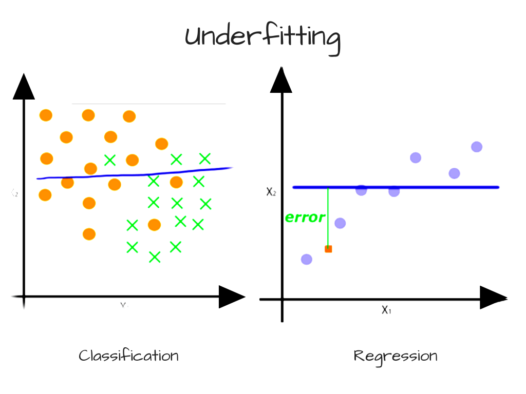
Another example would be continuous data that is polynomial in nature, with a model that can only represent linear relationships. In this case, it does not matter how much data we feed the model because it cannot represent the underlying relationship. To overcome error from bias, we need a more complex model.

Error due to Variance — Precision and Overfitting

Variance is a measure of how “sensitive” the model is to a subset of the training data.

When training a model, we typically use a limited number of samples from a larger population. If we repeatedly train a model with randomly selected subsets of data, we would expect its predictions to be different based on the specific examples given to it. Here variance is a measure of how much the predictions vary for any given test sample.

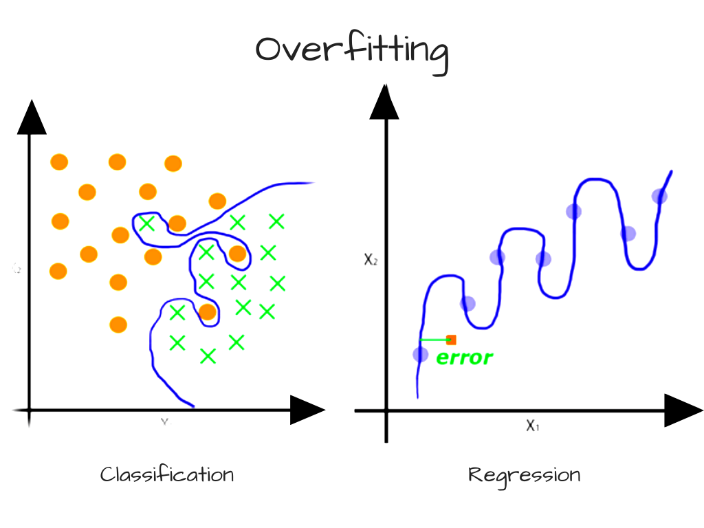
Some variance is normal, but too much variance indicates that the model is unable to generalize its predictions to the larger population. In such a scenario, the model will be very accurate for data that it’s already seen before. But it’ll perform poorly for unseen data points. High sensitivity to the training set is also known as overfitting, and generally occurs when the model is too complex. If your model is overfit, then you probably need to unburden it.

We can typically reduce the variability of a model’s predictions and increase precision by training on more data. If more data is unavailable, we can also control variance by limiting our model’s complexity.

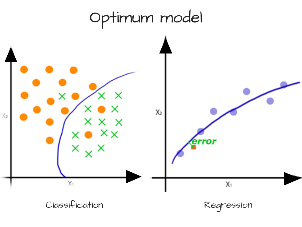
For the programmer, the challenge is to use the right type of algorithm which optimally solves the problem, while avoiding high bias or high variance. The reason is because:

• Increase in bias will decrease the variance
• Increase in variance will decrease the bias

This is also commonly referred to as The Bias-Variance tradeoff. Here’s a very nice detailed post on it that you could read later.

So unlike traditional programming, Machine Learning and Deep Learning problems can often involve a lot of trail-and-error based approaches when you’re trying to find the best model.

Now, you need to have a basic idea about some of the algorithms you can use to train your model. I won’t be diving into the mathematics or the lower-level implementation details, but this should be enough to give you some perspective.

Some of the most commonly used Machine Learning Algorithms:

Gaussian Naive Bayes

This technique has existed since the 1950s. It belongs to a family of algorithms called probabilistic classifiers or conditional probability, where it also assumes independence between features. Naive Bayes can be applied effectively for some classification problems, such as marking emails as spam or not spam, or classifying news articles.

Decision Trees

It is basically a tree-like data structure, which behaves like a flowchart. A Decision tree is a classification algorithm that uses tree-like data structures to model decisions and their possible outcomes. The way the algorithm works is:

• Place the best attribute of the dataset at the root of the tree.
• The nodes, or the place where a branch splits, is often called the “decision node.” It usually represents a test/conditional. (such as if it’s cloudy or sunny)
• The branches represent the outcome of each decision.
• The leaf nodes indicate the final outcome or the label (in classification problems), or a discrete value in regression problems.

Random Forests

When used alone, decision trees are prone to overfitting. However, random forests help by correcting the possible overfitting that could occur. Random forests work by using multiple decision trees — using a multitude of different decision trees with different predictions, a random forest combines the results of those individual trees to give the final outcomes.

Random forest applies an ensemble algorithm called bagging to the decision trees, which helps reduce variance and overfitting.

• Given a training set X = x1, …, xn with the labels/outcomes Y = y1, …, yn, bagging repeatedly (B times) selects a random sample with replacement of the training set
• Train decision trees with those samples
• Make the classifications by taking the majority vote of the classification trees

Apart from these, there are several other algorithms, such as Support Vector Machines, Ensemble methods and plenty of Unsupervised Learning methods. More on that later.

The training pipeline

First, we’ll need to prepare our data.

Data preparation

For the purposes of this tutorial, you’ll convert our regression problem into a classification problem. All wines with ratings less than 5 will fall under 0 (poor) category, wines with ratings 5 and 6 will be classified with the value 1 (average), and wines with 7 and above will be of great quality (2).

#Defining the splits for categories. 1–4 will be poor quality, 5–6 will be average, 7–10 will be great
bins = [1,4,6,10]

#0 for low quality, 1 for average, 2 for great quality
quality_labels=[0,1,2]
data['quality_categorical'] = pd.cut(data['quality'], bins=bins, labels=quality_labels, include_lowest=True)

#Displays the first 2 columns
display(data.head(n=2))

# Split the data into features and target label
quality_raw = data['quality_categorical']
features_raw = data.drop(['quality', 'quality_categorical'], axis = 1)

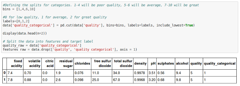
As you can see, there’s a new column called quality_categorical that classifies the quality ratings based on the range you chose earlier. You’ll use quality_categorical as the target values, and the rest as the features.

Next, you’ll create training and testing subsets for the data:

# Import train_test_split
from sklearn.model_selection import train_test_split

# Split the 'features' and 'income' data into training and testing sets
X_train, X_test, y_train, y_test = train_test_split(features_raw, quality_raw, test_size = 0.2,r andom_state = 0)

# Show the results of the split
print("Training set has {} samples.".format(X_train.shape[0]))
print("Testing set has {} samples.".format(X_test.shape[0]))

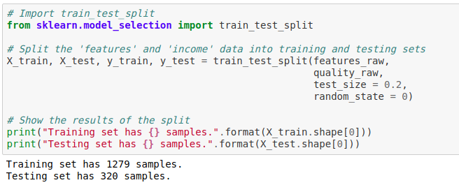
In the above code cell, we use the sklearn train_test_split method and give it our features data (X)and the target labels (y). It shuffles and dives our dataset into two parts — 80% of it is used for training and the remaining 20% is used for testing purposes.

Next, we’ll run our training on an algorithm and evaluate its performance.

Model training

You’ll need a function that’ll accept an ML algorithm of your choice, and the training and testing datasets. The function will run the training, and then will evaluate the performance of the algorithm using some performance metrics.

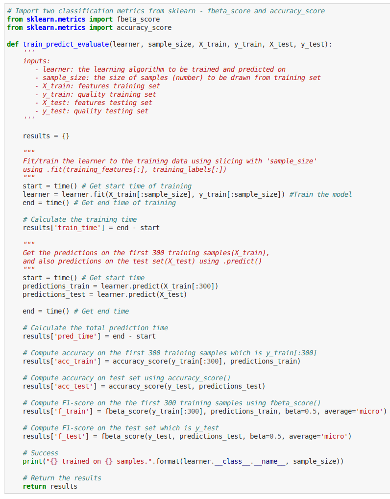
Finally, you’ll write a function where you’ll initialize any 3 algorithms of your choice, and run the training on each of them using the above function. You’ll then aggregate all the results, and then visualize them.

# Import any three supervised learning classification models from sklearn
from sklearn.naive_bayes import GaussianNB
from sklearn.tree import DecisionTreeClassifier
from sklearn.ensemble import RandomForestClassifier
#from sklearn.linear_model import LogisticRegression

# Initialize the three models
clf_A = GaussianNB()
clf_B = DecisionTreeClassifier(max_depth=None, random_state=None)
clf_C = RandomForestClassifier(max_depth=None, random_state=None)

# Calculate the number of samples for 1%, 10%, and 100% of the training data
# HINT: samples_100 is the entire training set i.e. len(y_train)
# HINT: samples_10 is 10% of samples_100
# HINT: samples_1 is 1% of samples_100

samples_100 = len(y_train)
samples_10 = int(len(y_train)*10/100)
samples_1 = int(len(y_train)*1/100)

# Collect results on the learners
results = {}
for clf in [clf_A, clf_B, clf_C]:
    clf_name = clf.__class__.__name__
    results[clf_name] = {}
    for i, samples in enumerate([samples_1, samples_10, samples_100]):
    results[clf_name][i] = \
    train_predict_evaluate(clf, samples, X_train, y_train, X_test, y_test)

#print(results)

# Run metrics visualization for the three supervised learning models chosen
vs.visualize_classification_performance(results)

The output will look like this:

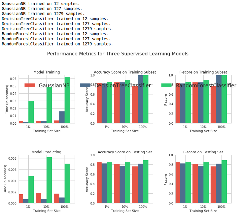
The above graph shows how well the algorithms performed in predictions. The first row shows the performance metrics on the training data, and the second row shows the metrics for the testing data (data which hasn’t been seen before). What do these performance metrics mean? Read on…

Performance Metrics for Classification Problems

Accuracy

Accuracy is by far the simplest and most commonly used performance metric. It is simply the ratio of correct predictions divided by the total data points. However, we might have scenarios in which our model might have really good accuracy, but it could fail to perform well for new unseen data points.

When is accuracy not a good indicator of performance?

Sometimes classification distributions in a data-set could be highly skewed. Meaning, the data could contain a whole lot of data-points for a few classes, and far fewer for the others. Let’s examine this with an example.

Let’s say that you have a data-set of 100 different emails. Amongst these emails, 10 of them are spam, while the other 90 aren’t. That means our data-set is skewed and unevenly distributed amongst the two classes — emails that are spam, and emails that aren’t spam.

Now, imagine that you trained a classifier using this data-set to predict whether a new email was spam or not. After evaluating its performance, you got a 90% accuracy rate. Sounds pretty good right? Not quite.

The reason is, the classifier could label or predict all 100 emails as “Not Spam”, and still have a great accuracy. In this case, it would have 90/100 = 0.9, or a 90% accuracy rate! But this classifier is of no use for us, since it’s always going to classify every email as not spam.

So, accuracy is not always a good indicator of performance. There are other metrics that can help you evaluate your models better in certain situations:

Precision

Precision tells us what proportion of messages classified as spam were actually were spam. It is a ratio of true positives (emails classified as spam, and which are actually spam) to all positives (all emails classified as spam, irrespective of whether that was the correct classification). In other words, it is the ratio of True Positives/(True Positives + False Positives).

Recall

Recall or sensitivity tells us what proportion of messages that actually were spam were classified by us as spam. It is a ratio of true positives (words classified as spam, and which are actually spam) to all the words that were actually spam (irrespective of whether we classified them correctly). It is given by the formula — True Positives/(True Positives + False Negatives)

Now, for our classifier which has a 90% accuracy rate, what would its precision and recall be? Let’s see — its True Positives are 0, False Positives are 0, and False Negatives are 10. Plugging these into our formulae, our classifier has precision and recall values of 0 — pretty abysmmal scores! Doesn’t look so great now, does it?

F1 Score

The F1 Score is the harmonic average of precision and recall. It’s given by the formula:

If you set the value of β to be higher, more emphasis is placed on precision.

---

Now, let’s have a look at how well our ML algorithms performed once again:

From these results, we can see that the performance of Gaussian Naive Bayes isn’t as great as that of Decision Tree or Random Forests.

Why do you think it fails to perform as well as the other algorithms? (Hint: feel free to scroll up and read the explanation of Gaussian Naive Bayes once more!)

Feature Importances

Some of the classification algorithms that scikit-learn provides, come with a feature importance attribute. Using this attribute, you can see the importance of each feature by its relative ranks when making predictions, based on the chosen algorithm.

Random Forest Classifier in scikit-learn has a .feature_importance_ attribute, so you could use the same classifier or choose an another one.

# Import a supervised learning model that has 'feature_importances_'
model = RandomForestClassifier(max_depth=None, random_state=None)

# Train the supervised model on the training set using .fit(X_train, y_train)
model = model.fit(X_train, y_train)

# Extract the feature importances using .feature_importances_
importances = model.feature_importances_

print(X_train.columns)
print(importances)

# Plot
vs.feature_plot(importances, X_train, y_train)

This will give you the following relative rankings:

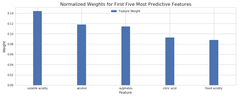
As you can clearly see, the graph shows five most important features that determine how good a wine is. Alcohol content and volatile acidity levels seem to be the most influential factors, followed by sulphates, citric acid and fixed acidity levels.

Hyperparameter Tuning and Optimization

As you might have noticed, Machine Learning (or even Deep Learning, for that matter) is related to Data Science. Like any other science, it begins with some prior observations. You then make a hypothesis, run some experiments, and then analyze how closely they replicate the earlier observations. This is also known as The Scientific Method. It’s similar to the engineering process as well.

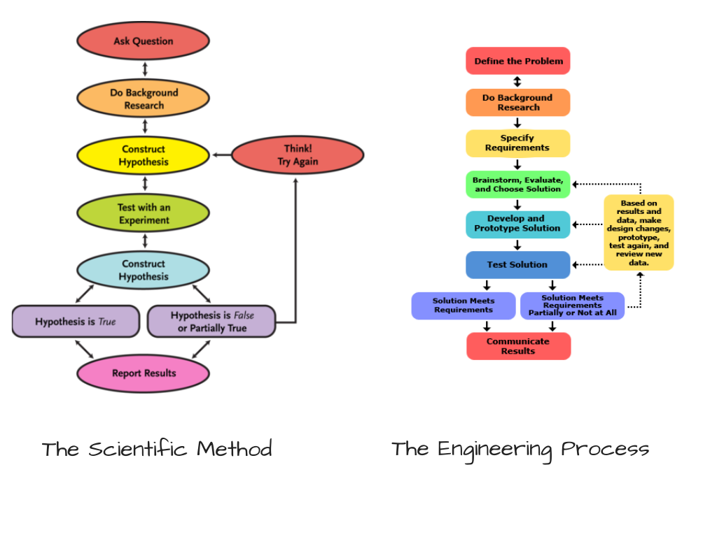
A hypothesis can also be thought of as an “assumption”. While building our classifier, we first hypothesized a bunch of algorithms, which in our opinion would work well. But our hypothesis could be wrong, too. We still aren’t sure whether they are “tailored” or “tuned” well. Often, we need to tune our hypotheses to see if they can be made better.

While choosing our Machine Learning models, we made initial assumptions about some of their hyperparameters. A hyperparameter is a special type of configuration variable whose value cannot be directly calculated using the data-set. It’s the job of the data scientist or machine learning engineer to experiment and figure out the optimal values of these hyperparameters. This process is called hyperparameter tuning.

Now, for our Random Forest Algorithm, what might its hyperparameters be?

• Number of decision trees in the forest
• The number of features to consider while looking for the best split in a tree
• The maximum depth of the tree, or the longest path from the root to its leaf

For these hyperparameters, our random forest classifier used default values that come bundled within the scikit-learn APIs.

Now, wouldn’t it take a long time for us to repeatedly train, analyze and record the performance of an algorithm for different values of a bunch of hyper-parameters?

Yes it would! Lucky for us, scikit-learn provides a very convenient API that does the heavy lifting for us. We can specify different values for our hyperparameters in a “grid”, and scikit-learn’s GridSearchCV API would train and run cross validation on all possible combinations of these hyperparameters and give us the optimum configuration. This way, we don’t manually have to run so many iterations.

Run the code in the next cell block to tune your model:

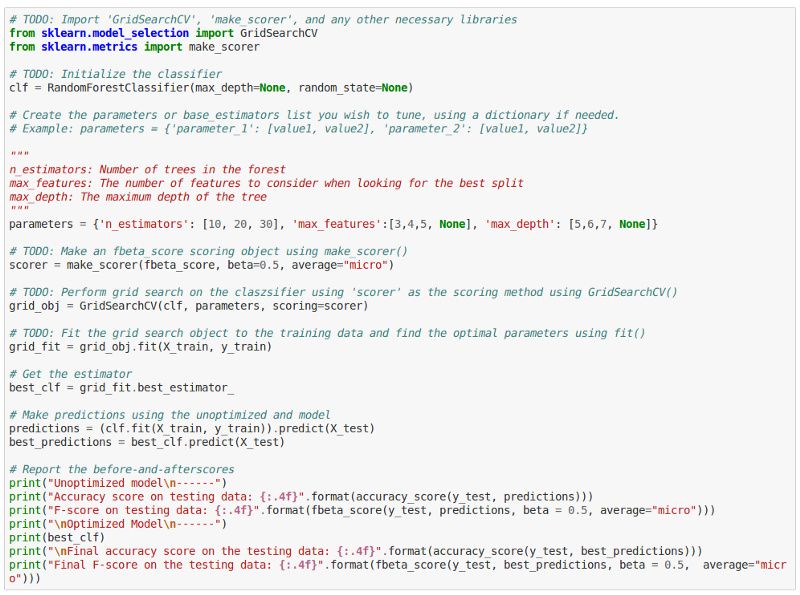
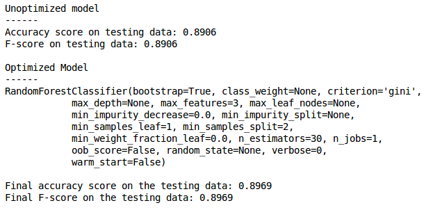
And done. You can see that the performance of our model has in fact slightly increased!

Using your model for Predictions

Finally, you can test your model out by giving it a bunch of values for various features, and see what it predicts:

Congratulations! You have successfully built your very own machine learning classifier that can predict good wines and bad wines. I hope you had fun solving this exercise. Now sit back, have a drink, and revel in your knowledge of machine learning!

Some questions that you should ponder upon:

• Is your classifier better suited for detecting average wines, or better equipped to detect good wines? What do you think could be the reason?
• Would you recommend your classifier to a wine manufacturer? If yes, then why? If no, why not?
• How well will your model perform if you trained it using regresion techniques, instead of classification?

What next?

• Try solving this exercise with the white wines data-set
• Head over to Kaggle, explore different data-sets, and work on one that you find interesting.
• Write an API service that uses your machine learning models, and make a nice web or mobile app

Finally, you should definitely check out these —

Resources

• A beginner’s guide to AI and ML
• Machine Learning Mastery
• Intro to Machine Learning — Udacity
• A Visual Introduction to Machine Learning
• A tour of Machine Learning Algorithms
• 40 Interview Questions asked at Data Science and Machine Learning Startups

Until then, Valar Alcoholis! May you achieve awesome F1 Scores for all your re(solutions) this year.

If you have any questions, or if you’d like to have a certain topic covered — feel free to comment or discuss below! What would you like to learn next?